Analyzing Multistate Trajectory Files with openfe-analysis

This notebook demonstrates how to load, align, and analyze multistate trajectory files produced by OpenFE’s free energy protocols. We cover two protocols:

• Relative Hybrid Topology Protocol (RBFE): a single hybrid ligand is used to represent both end states. The trajectory contains one ligand per frame.

• Separated Topologies Protocol (SepTop): both ligands are present simultaneously throughout the simulation. The trajectory contains two physically distinct ligands per frame.

For each protocol we analyse both the complex leg (protein + ligand) and the solvent leg (ligand only) separately, computing structural metrics including ligand RMSD, ligand centre-of-mass drift, and protein 2D RMSD to assess simulation quality.

Removal of periodic boundary conditions and alignment operations

Before computing any RMSD-based metric, trajectories must be preprocessed to remove periodic boundary condition (PBC) artefacts and rigid-body motion. openfe-analysis handles all of this automatically by applying a series of MDAnalysis Universe Transformations on-the-fly as frames are read:

1. Unwrap (unwrap): Makes each molecule whole by repairing splits across periodic boundaries.

2. Image (ClosestImageShift): Shifts molecules into the same periodic image. In a complex simulation the ligand may appear in a neighbouring periodic image relative to the protein. In SepTop, each ligand must be imaged independently, since they can cross periodic boundaries at different times.

3. Align (Aligner): Aligns all frames to a common reference (the first frame) by minimizing the protein Cα RMSD, removing overall translational and rotational motion so that structural changes reflect internal structural changes only.

For solvent leg simulations, NoJump is used instead of unwrap and ClosestImageShift to track the ligand’s centre-of-mass motion continuously across frames, preventing it from jumping between periodic images.

Structural metrics

The following metrics are computed for each lambda state. The complex and solvent legs differ in which analyses are meaningful:

Complex leg (protein + ligand)

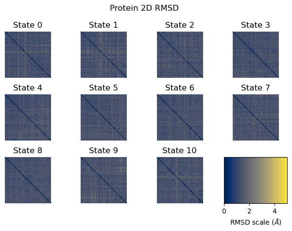
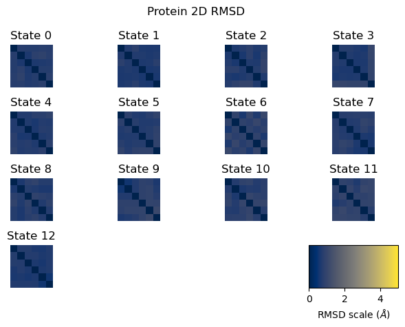
• 2D Protein RMSD: a pairwise RMSD matrix computed between all analyzed frame pairs. A well-behaved simulation shows a uniform low-RMSD matrix. High RMSD values between certain frame pairs (visible as bright patches) suggest the protein visited structurally distinct conformations during the simulation.

• Ligand RMSD: measures how much the ligand moves relative to its pose in the binding site at the start of the production simulation. Values above ~5 Å may indicate the ligand has shifted significantly or left the binding site. For SepTop, a symmetry-corrected RMSD is used instead, which accounts for equivalent atom orderings in symmetric molecules (e.g. flipping a phenyl ring) that would otherwise give a non-zero RMSD for physically identical poses. For the hybrid topology protocol, a standard mass-weighted RMSD is used as symmetry correction requires additional handling for hybrid topologies.

• Ligand COM drift: measures how far the ligand’s centre-of-mass has moved from its position at the start of the production phase. Unlike RMSD,this is sensitive only to translational movement and ignores rotations which is useful for detecting whether the ligand has drifted out of the binding site. Values above ~5 Å may indicate the ligand is leaving the binding site. Note that any drift that occurred during equilibration will not be captured by this metric.

Solvent leg (ligand only)

• Ligand RMSD: same as above but without protein context.

For SepTop, all ligand-based metrics are computed independently for both ligand A and ligand B.

Download tutorial data

First, download the example trajectory data used throughout this notebook. This may take a few minutes due to the file sizes.

%%bash

# Hybrid topology
wget --show-progress "https://zenodo.org/records/20442933/files/openfe_analysis_skipped.tar.gz" -nc
tar -xzf openfe_analysis_skipped.tar.gz

# SepTop
wget --show-progress "https://zenodo.org/records/20507106/files/septop_structural_results.zip" -nc
unzip -n septop_structural_results.zip

File 'openfe_analysis_skipped.tar.gz' already there; not retrieving.

File 'septop_structural_results.zip' already there; not retrieving.

Archive:  septop_structural_results.zip

Imports

import pathlib

import matplotlib.pyplot as plt
import MDAnalysis as mda
import netCDF4 as nc
import numpy as np
from rdkit.Chem import SDMolSupplier

from openfe_analysis.rmsd import (
    LigandCOMDrift,
    Protein2DRMSD,
    RMSDAnalysis,
    SymmetryCorrectedLigandRMSD,
)
from openfe_analysis.utils.apply_transformations import (
    apply_complex_alignment_transformations,
    apply_ligand_alignment_transformations,
)
from openfe_analysis.utils.universe_utils import create_universe_single_state

Let’s define the paths to the downloaded tutorial data that we will use throughout this notebook.

rfe_dir = pathlib.Path("openfe_analysis_skipped")
septop_dir = pathlib.Path("septop_structural_results")

Relative Hybrid Topology Protocol

Complex leg

Here we compute the protein 2D RMSD, ligand RMSD, and ligand COM drift for the complex leg.

Load trajectory and topology

The PDB file provides the topology (atom names, residues, bonds) and the .nc file contains the multistate trajectory, with one set of coordinates per lambda state per frame.

rfe_complex_pdb = rfe_dir / "hybrid_system.pdb"
rfe_complex_nc = rfe_dir / "simulation.nc"

Compute structural metrics across all lambda states

We loop over all lambda states, loading each as a separate MDAnalysis Universe using create_universe_single_state so that alignment transformations applied to one state do not affect another. We also compute a skip rate upfront to target approximately 500 frames per state, keeping computation time manageable for long trajectories.

rfe_lig_rmsd = []
rfe_lig_com_drift = []
rfe_prot_2d_rmsd = []
rfe_time_ps = None
    
protein_selection = "protein and name CA"
ligand_selection = "resname UNK"
with nc.Dataset(rfe_complex_nc) as ds:
    n_lambda = ds.dimensions["state"].size

    # Account for the position skip rate set during the simulation
    if hasattr(ds, "PositionInterval"):
        n_frames = len(range(0, ds.dimensions["iteration"].size, ds.PositionInterval))
    else:
        n_frames = ds.dimensions["iteration"].size

    # Compute a skip rate to target ~500 frames of output per state
    # max against 1 to avoid skip=0 for very short trajectories
    skip = max(n_frames // 500, 1)

    u_top = mda.Universe(rfe_complex_pdb)
    
    # Loop over all lambda states
    for state_idx in range(n_lambda):
        # Create a separate Universe for each lambda state
        universe = create_universe_single_state(u_top._topology, ds, state_idx)
        prot = universe.select_atoms(protein_selection)
        lig = universe.select_atoms(ligand_selection)
        
        # Add PBC-handling and alignment transformations to the Universe
        apply_complex_alignment_transformations(universe, protein=prot, ligands=[lig])

        # Calculate the protein 2D RMSD
        protein_2d_rmsd = Protein2DRMSD(prot).run(step=skip)
        rfe_prot_2d_rmsd.append(protein_2d_rmsd.results.rmsd2d)

        # Calculate the ligand RMSD
        ligand_rmsd = RMSDAnalysis(lig, mass_weighted=True).run(step=skip).results.rmsd
        rfe_lig_rmsd.append(ligand_rmsd)

        # Calculate the Ligand COM drift
        ligand_com_drift = LigandCOMDrift(lig).run(step=skip).results.com_drift
        rfe_lig_com_drift.append(ligand_com_drift)
        
        # Record the time axis from the first state
        if rfe_time_ps is None:
            rfe_time_ps = (
                np.arange(len(universe.trajectory))[::skip] * universe.trajectory.dt
            )

Plot results

Each line represents one lambda state. Consistent profiles across states indicate a stable, well-behaved simulation. Large deviations in specific states may indicate sampling problems or instabilities.

from openfe_analysis.utils.plotting import (
    plot_2D_rmsd,
    plot_ligand_RMSD,
    plot_ligand_COM_drift,
)

Protein 2D RMSD

The 2D RMSD is computed as a pairwise RMSD between all analyzed frame pairs, after centering and rotational superposition. A well-behaved simulation shows a uniform low-RMSD matrix (blue tones). High RMSD values between certain frame pairs (visible as bright patches) suggest the protein visited structurally distinct conformations during the simulation.

fig = plot_2D_rmsd(rfe_prot_2d_rmsd)
plt.show()

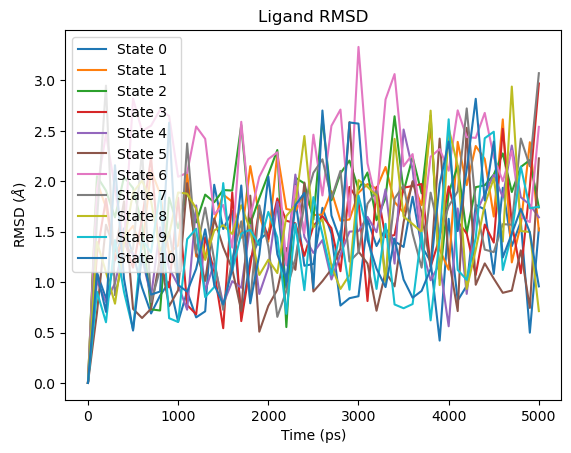
Ligand RMSD

The first frame RMSD is always zero, as all frames are measured relative to the ligand position at the start of the production phase. Values above ~5 Å may indicate the ligand has shifted significantly. Note that dummy atoms are included in this RMSD calculation. As dummy atoms do not interact with the environment they can move more, potentially inflating the RMSD value without reflecting any real change in the ligand pose.

fig = plot_ligand_RMSD(rfe_time_ps, rfe_lig_rmsd)
plt.show()

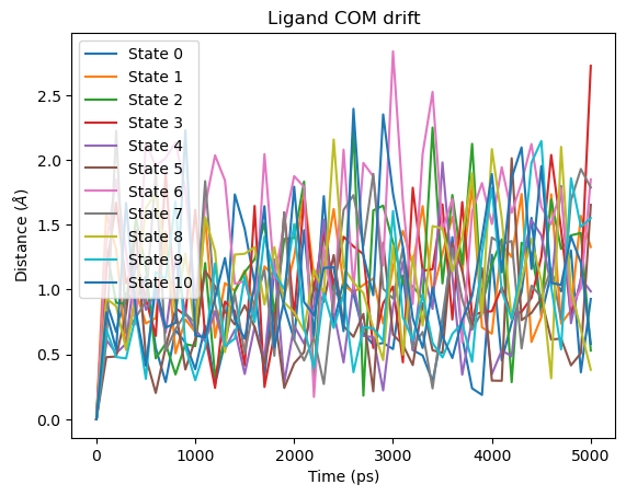
Ligand COM drift

Values above ~5 Å may indicate the ligand is drifting out of the binding site.

Note that the reference position is the ligand’s position at the start of the production phase, not the original binding pose. If the ligand drifted from the binding site during equilibration, this will not be captured.

fig = plot_ligand_COM_drift(rfe_time_ps, rfe_lig_com_drift)
plt.show()

Separated Topologies (SepTop)

SepTop Complex leg

As with the RBFE complex leg, we compute the protein 2D RMSD, ligand RMSD, and ligand COM drift, here for both ligand A and ligand B independently.

Load trajectory and topology

In addition to the topology and trajectory files, we load the RDKit molecules for each ligand, which are needed for the symmetry-corrected RMSD calculation.

septop_complex_pdb = septop_dir / "complex" / "alchemical_system.pdb"
septop_complex_nc_file = septop_dir / "complex" / "complex.nc"

rdmol_A = SDMolSupplier(str(septop_dir / "complex" / "ligand_A.sdf"), removeHs=False)[0]
rdmol_B = SDMolSupplier(str(septop_dir / "complex" / "ligand_B.sdf"), removeHs=False)[0]

Getting ligand indices

In a real SepTop calculation, the ligand indices are stored in the protocol output JSON and can be extracted from there. For this tutorial we derive them directly from the topology by residue name, which works because the two ligands have distinct residue indices within the same residue name UNK.

u_tmp = mda.Universe(septop_complex_pdb)

# Select all UNK residues — in a SepTop system these are the two ligands
unk_residues = u_tmp.select_atoms("resname UNK").residues

septop_ligand_A_indices = unk_residues[0].atoms.indices.tolist()
septop_ligand_B_indices = unk_residues[1].atoms.indices.tolist()

Compute structural metrics across all lambda states

As with the hybrid topology RBFE complex leg, we loop over all lambda states loading each as a separate Universe. Both ligands are passed as separate AtomGroups to apply_complex_alignment_transformations so that each is imaged independently relative to the protein. SymmetryCorrectedLigandRMSD is used for both ligands since SepTop preserves the full atom identity of each molecule.

septop_prot_rmsds = []
septop_lig_A_rmsds = []
septop_lig_B_rmsds = []
septop_lig_A_drifts = []
septop_lig_B_drifts = []
septop_prot_2d_rmsds = []
septop_time_ps = None

with nc.Dataset(septop_complex_nc_file) as ds:
    n_lambda = ds.dimensions["state"].size

    # Account for the position skip rate.
    if hasattr(ds, "PositionInterval"):
        n_frames = len(range(0, ds.dimensions["iteration"].size, ds.PositionInterval))
    else:
        n_frames = ds.dimensions["iteration"].size

    # find skip that would give ~500 frames of output
    # max against 1 to avoid skip=0 case
    septop_skip = max(n_frames // 500, 1)

    u_top = mda.Universe(septop_complex_pdb)
    
    for state_idx in range(n_lambda):
        
        # Create an MDAnalysis universe for this state
        universe = create_universe_single_state(u_top._topology, ds, state_idx)
        prot = universe.select_atoms(protein_selection)
        lig_A = universe.atoms[septop_ligand_A_indices]
        lig_B = universe.atoms[septop_ligand_B_indices]

        # Remove PBC artifacts and align frames
        apply_complex_alignment_transformations(universe, protein=prot, ligands=[lig_A, lig_B])

        # Calculate the protein 2D RMSD
        septop_prot_2d_rmsds.append(
            Protein2DRMSD(prot).run(step=septop_skip).results.rmsd2d
        )

        # Calculate the symmetry corrected RMSD
        septop_lig_A_rmsds.append(
            SymmetryCorrectedLigandRMSD(lig_A, rdmol=rdmol_A)
            .run(step=septop_skip).results.rmsd
        )
        septop_lig_B_rmsds.append(
            SymmetryCorrectedLigandRMSD(lig_B, rdmol=rdmol_B)
            .run(step=septop_skip).results.rmsd
        )
        # Calculate the Ligand COM drift
        septop_lig_A_drifts.append(
            LigandCOMDrift(lig_A).run(step=septop_skip).results.com_drift
        )
        septop_lig_B_drifts.append(
            LigandCOMDrift(lig_B).run(step=septop_skip).results.com_drift
        )
        

        if septop_time_ps is None:
            septop_time_ps = (
                np.arange(len(universe.trajectory))[::septop_skip] * universe.trajectory.dt
            )

Plot results

As with the RBFE complex leg, each line represents one lambda state. Results are shown separately for ligand A and ligand B.

Protein 2D RMSD

fig = plot_2D_rmsd(septop_prot_2d_rmsds)
plt.show()

Ligand RMSD

# Ligand A RMSD
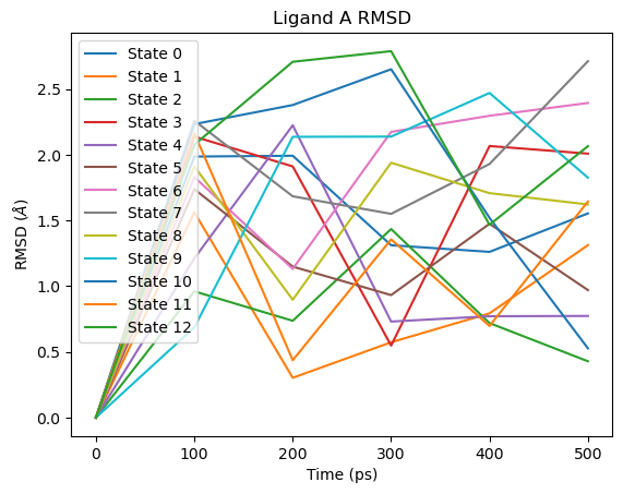
fig = plot_ligand_RMSD(septop_time_ps, septop_lig_A_rmsds)
fig.axes[0].set_title("Ligand A RMSD")
plt.show()

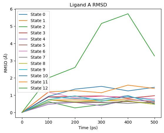
The large RMSD spike visible towards the end of the simulation corresponds to the fully decoupled end state (State 12), where ligand A has no interactions with the environment and is only held in the binding site by Boresch-style restraints. This is expected behaviour and does not indicate a problem with the simulation.

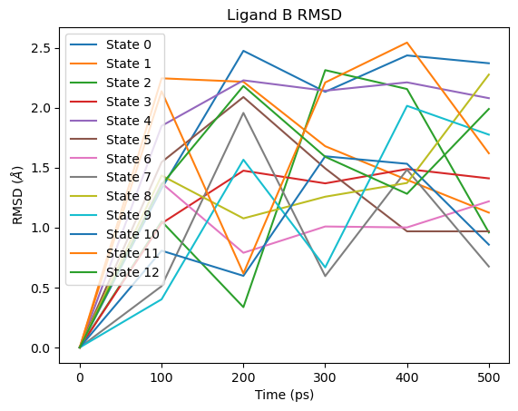
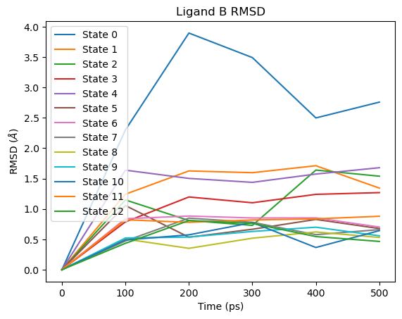
For ligand B the pattern is reversed: the large RMSD spike appears at the beginning of the lambda schedule (State 0), corresponding to the end state where ligand B has no interactions with the environment:

# Ligand B RMSD
fig = plot_ligand_RMSD(septop_time_ps, septop_lig_B_rmsds)
fig.axes[0].set_title("Ligand B RMSD")
plt.show()

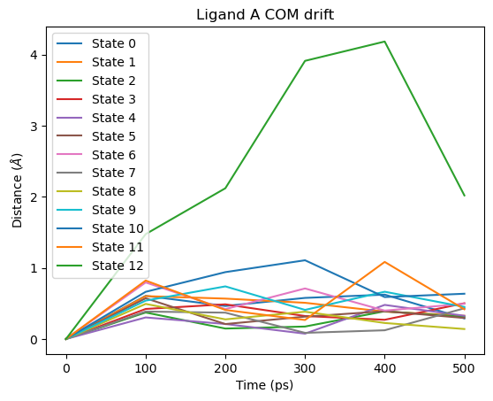
Ligand COM drift

# Ligand A COM drift
fig = plot_ligand_COM_drift(septop_time_ps, septop_lig_A_drifts)
fig.axes[0].set_title("Ligand A COM drift")
plt.show()

# Ligand B COM drift
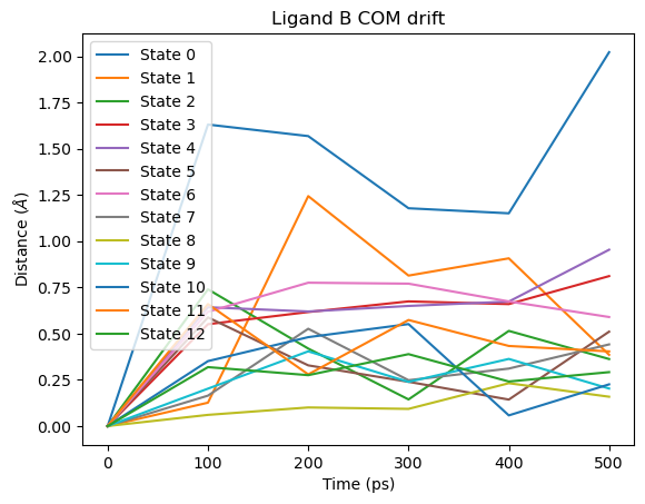
fig = plot_ligand_COM_drift(septop_time_ps, septop_lig_B_drifts)
fig.axes[0].set_title("Ligand B COM drift")
plt.show()

SepTop Solvent leg

In the solvent leg only the two ligands are present, without protein. We compute the ligand RMSD for both ligand A and ligand B independently.

Load trajectory and topology

septop_solvent_pdb = septop_dir / "solvent" / "alchemical_system.pdb"
septop_solvent_nc_file = septop_dir / "solvent" / "solvent.nc"

Getting ligand indices

In the solvent leg, both ligands appear as a single UNK residue in the topology. We use the atom counts derived from the complex leg to slice the solvent UNK atoms into ligand A and ligand B, and verify the expected total atom count with an assert before proceeding.

n_atoms_A = len(septop_ligand_A_indices)
n_atoms_B = len(septop_ligand_B_indices)

u_tmp_solvent = mda.Universe(septop_solvent_pdb)
unk_solvent = u_tmp_solvent.select_atoms("resname UNK")
print(f"Solvent UNK atoms: {unk_solvent.n_atoms}")
print(f"Expected: {n_atoms_A} (ligand A) + {n_atoms_B} (ligand B) = {n_atoms_A + n_atoms_B}")

assert unk_solvent.n_atoms == n_atoms_A + n_atoms_B, (
    f"Unexpected atom count: {unk_solvent.n_atoms}"
)

# Ligand A comes first, ligand B second
septop_solvent_ligand_A_indices = unk_solvent.indices[:n_atoms_A].tolist()
septop_solvent_ligand_B_indices = unk_solvent.indices[n_atoms_A:].tolist()

print(f"Ligand A indices: {septop_solvent_ligand_A_indices[0]}–{septop_solvent_ligand_A_indices[-1]}")
print(f"Ligand B indices: {septop_solvent_ligand_B_indices[0]}–{septop_solvent_ligand_B_indices[-1]}")

Solvent UNK atoms: 75
Expected: 37 (ligand A) + 38 (ligand B) = 75
Ligand A indices: 0–36
Ligand B indices: 37–74

Compute structural metrics across all lambda states

In the solvent leg we create a separate Universe for each ligand. This is necessary because apply_ligand_alignment_transformations uses NoJump to prevent the ligand from jumping between periodic images by tracking its centre-of-mass motion continuously across frames. If both ligands shared a Universe, the transformation applied to one would affect the coordinate frame seen by the other.

septop_solvent_lig_A_rmsds = []
septop_solvent_lig_B_rmsds = []
septop_solvent_time_ps = None

with nc.Dataset(septop_solvent_nc_file) as ds:
    n_lambda = ds.dimensions["state"].size
    if hasattr(ds, "PositionInterval"):
        n_frames = len(range(0, ds.dimensions["iteration"].size, ds.PositionInterval))
    else:
        n_frames = ds.dimensions["iteration"].size
    septop_solvent_skip = max(n_frames // 500, 1)

    u_top_solvent = mda.Universe(septop_solvent_pdb)
    
    for state_idx in range(n_lambda):
        # Ligand A: independent universe and alignment
        universe_A = create_universe_single_state(
            u_top_solvent._topology, ds, state_idx
        )
        lig_A = universe_A.atoms[septop_solvent_ligand_A_indices]
        apply_ligand_alignment_transformations(universe_A, ligand=lig_A)
        septop_solvent_lig_A_rmsds.append(
            SymmetryCorrectedLigandRMSD(lig_A, rdmol=rdmol_A)
            .run(step=septop_solvent_skip).results.rmsd
        )
    
        # Ligand B: separate universe so NoJump tracks it independently
        universe_B = create_universe_single_state(
            u_top_solvent._topology, ds, state_idx
        )
        lig_B = universe_B.atoms[septop_solvent_ligand_B_indices]
        apply_ligand_alignment_transformations(universe_B, ligand=lig_B)
        septop_solvent_lig_B_rmsds.append(
            SymmetryCorrectedLigandRMSD(lig_B, rdmol=rdmol_B)
            .run(step=septop_solvent_skip).results.rmsd
        )
    
        if septop_solvent_time_ps is None:
            septop_solvent_time_ps = (
                np.arange(len(universe_A.trajectory))[::septop_solvent_skip]
                * universe_A.trajectory.dt
            )

Plot results

# Ligand A RMSD
fig = plot_ligand_RMSD(septop_solvent_time_ps, septop_solvent_lig_A_rmsds)
fig.axes[0].set_title("Ligand A RMSD")
plt.show()

# Ligand B RMSD
fig = plot_ligand_RMSD(septop_solvent_time_ps, septop_solvent_lig_B_rmsds)
fig.axes[0].set_title("Ligand B RMSD")
plt.show()